Branchless Lomuto Partitioning

A partition function accepts as input an array of elements, and a function returning a bool (a predicate) which indicates if an element should be in the first, or second partition. Then it returns two arrays, the two partitions:

def partition(v, pred):
    first = [x for x in v if pred(x)]
    second = [x for x in v if not pred(x)]
    return first, second

This can actually be done without needing any extra memory beyond the original array. An in-place partition algorithm reorders the array such that all the elements for which pred(x) is true come before the elements for which pred(x) is false (or vice versa - it doesn’t really matter). Finally by returning how many elements satisfied pred(x) to the caller they can then logically split the array in two slices. This scheme is used in C++’s std::partition for example.

In-place partition algorithms

There are many possible variations / implementations of in-place partition algorithms, but they usually follow one of two schools: Hoare or Lomuto, named after their original inventors Tony Hoare (the inventor of quicksort), and Nico Lomuto.

Hoare

In Hoare-style partition algorithms you have two iterators scanning the array, one left-to-right ($i$) and one right-to-left ($j$). The former tries to find elements that belong on the right, and the latter tries to find elements that belong on the left. When both iterators have found an element, you swap them, and continue. When the iterators cross each other you are done.

def hoare_partition(v, pred):
    i = 0       # Loop invariant: all(pred(x) for x in v[:i])
    j = len(v)  # Loop invariant: all(not pred(x) for x in v[j:])
    while True:
        while i < j and pred(v[i]): i += 1
        j -= 1
        while i < j and not pred(v[j]): j -= 1
        if i >= j: return i
        v[i], v[j] = v[j], v[i]
        i += 1

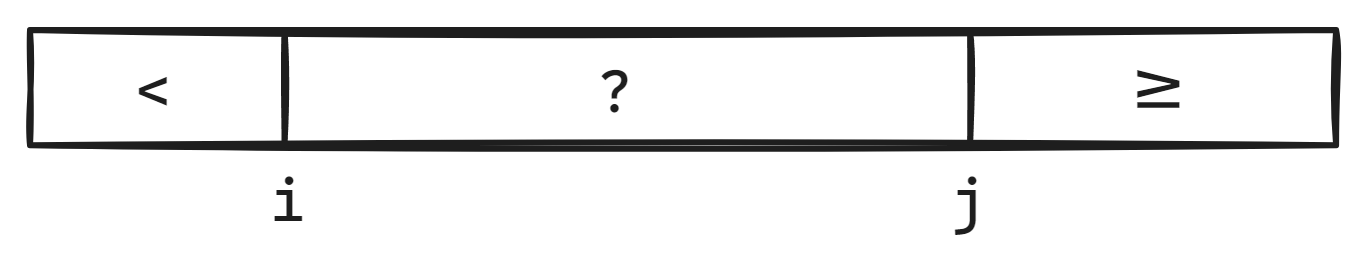
The loop invariant can visually be seen as such (using the symbols $<$ and $\geq$ for the predicate outcomes, as is usual in sorting):

Doing this efficiently is perhaps an article for another day, if you are curious you can check out the paper BlockQuicksort: How Branch Mispredictions don’t affect Quicksort by Stefan Edelkamp and Armin Weiß, which is the technique I implemented in pdqsort. Another take on the same idea is found in bitsetsort. Key here is that it can be done branchlessly. A branch is a point at which the CPU has to make a choice of which code to run. The most recognizable form of a branch is the if statement, but there are others (e.g. while conditions, calling a function from a lookup table, short-circuiting logical operators).

To cut a long story short, CPUs try to predict which piece of code it should run next and already starts doing it even before it knows if the code it is sending down the pipeline is the right choice. This is great in most cases as most branches are easy to predict, but it does incur a penalty when the prediction was wrong, as the CPU needs to stop, go back and restart from the right point once it realizes it was wrong (which can take a while).

Especially in sorting when the outcomes of comparisons are ideally unpredictable (the more unpredictable the outcome of a comparison, the more informative getting the answer is), it can thus be advisable to avoid branching on comparisons altogether.

Lomuto

In Lomuto-style partition algorithms the following invariant is followed:

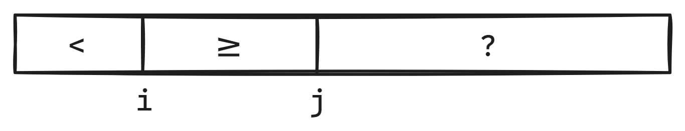
That is, there is a single iterator scanning the array from left-to-right ($j$). If the element is found to belong in the left partition, it is swapped with the first element of the right partition (tracked by $i$), otherwise it is left where it is.

def lomuto_partition(v, pred):
    i = 0  # Loop invariant: all(pred(x) for x in v[:i])
    j = 0  # Loop invariant: all(not pred(x) for x in v[i:j])
    while j < len(v):
        if pred(v[j]):
            v[i], v[j] = v[j], v[i]
            i += 1
        j += 1

    return i

This article is focused on optimizing this style of partition.

Branchless Lomuto

A few years ago I read a post by Andrei Alexandrescu which discusses a branchless variant of the Lomuto partition. Its inner loop (in C++) looks like this:

for (; read < last; ++read) {
    auto x = *read;
    auto smaller = -int(x < pivot);
    auto delta = smaller & (read - first);
    first[delta] = *first;
    read[-delta] = x;
    first -= smaller;
}

At the time I was not overly impressed, as it does a lot of arithmetic to make the loop branchless, so I disregarded it. A while back my friend Lukas Bergdoll approached me with a new partition algorithm which was doing quite well in his benchmarks, which I recognized as being a variant of Lomuto. I then found a way the algorithm could be restructured without using conditional move instructions, which made it perform better still. I will present this algorithm now.

Simple version

First, a simplified variant which will make the more optimized variant much more readily understood:

def branchless_lomuto_partition_simplified(v, pred):
    i = 0  # Loop invariant: all(pred(x) for x in v[:i])
    j = 0  # Loop invariant: all(not pred(x) for x in v[i:j])
    while j < len(v):
        v[i], v[j] = v[j], v[i]
        i += int(pred(v[i]))
        j += 1

    return i

This is actually quite similar to the original lomuto_partition, except we now always unconditionally swap, and replace the conditional increment of $i$ with an if statement by simply converting the boolean condition to an integer and adding it to $i$.

To visualize this, the state of the array looks like this after the unconditional swap:

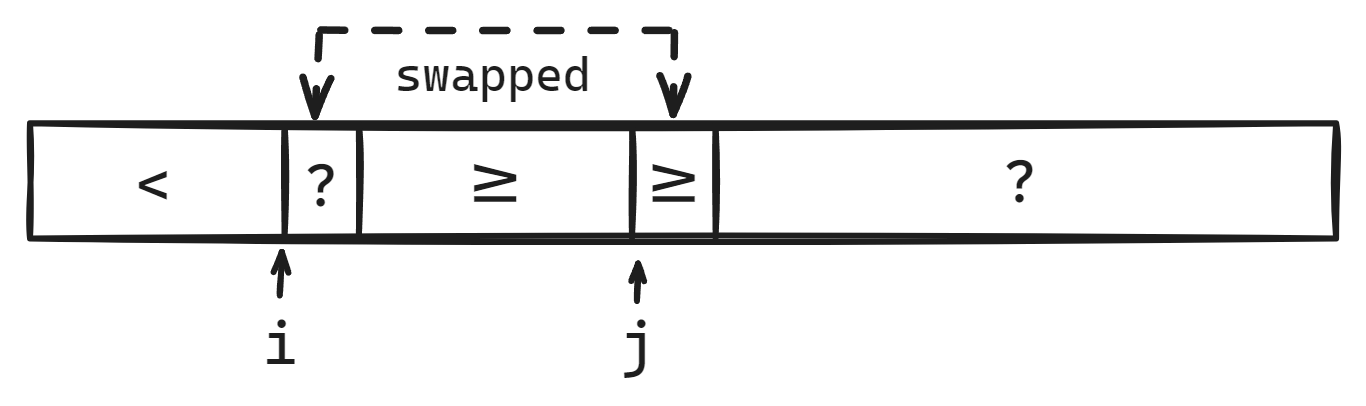
From this it should be pretty clear that incrementing $i$ if the predicate is true (corresponding to $v[i] < p$ for sorting) and unconditionally incrementing $j$ restores our Lomuto loop invariant. The only corner case is when ${i = j},$ but then the swap is a no-op and the algorithm remains correct.

Eliminating swaps

Swaps are equivalent to three moves, but by restructuring the algorithm we can get away with two moves per iteration. The trick is to introduce a gap in the array by temporarily moving one of the elements out of the array.

def branchless_lomuto_partition(v, pred):
    if len(v) == 0: return 0

    tmp = v[0]
    i = 0  # Loop invariant: all(pred(x) for x in v[:i])
    j = 0  # Loop invariant: all(not pred(x) for x in v[i:j])
    while j < len(v) - 1:
        v[j] = v[i]
        j += 1
        v[i] = v[j]
        i += pred(v[i])

    v[j] = v[i]
    v[i] = tmp
    i += pred(v[i])
    return i

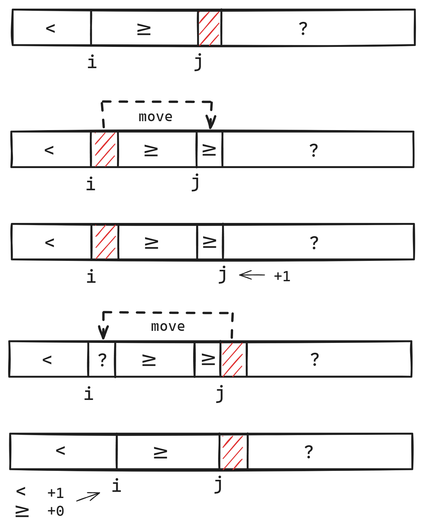
This is our new branchless Lomuto partition algorithm. Its inner loop is incredibly tight, involving only two moves, one predicate evaluation and two additions. A full visualization of one iteration of the algorithm (the striped red area indicates the gap in the array):

We can now compare the assembly of the tight inner loops of Andrei Alexandrescu’s branchless Lomuto partition and ours:

.alexandrescu:
    mov     edi, DWORD PTR [rdx]
    mov     rsi, rdx
    mov     ebp, DWORD PTR [rax]
    cmp     edi, r8d
    setb    cl
    sub     rsi, rax
    sar     rsi, 2
    test    cl, cl
    cmove   rsi, rbx
    sal     rcx, 63
    sar     rcx, 61
    mov     DWORD PTR [rax+rsi*4], ebp
    lea     r11, [0+rsi*4]
    mov     rsi, rdx
    add     rdx, 4
    sub     rsi, r11
    sub     rax, rcx
    mov     DWORD PTR [rsi], edi
    cmp     rdx, r10
    jb      .alexandrescu

.orlp:
    lea     rdi, [r8+rax*4]
    mov     ecx, DWORD PTR [rdi]
    mov     DWORD PTR [rdx], ecx
    mov     ecx, DWORD PTR [rdx+4]
    cmp     ecx, r9d
    mov     DWORD PTR [rdi], ecx
    adc     rax, 0
    add     rdx, 4
    cmp     rdx, r10
    jne     .orlp

Half the instruction count! A neat trick the compiler did is translate the addition of the boolean result of the predicate (which is just a comparison here) to adc rax, 0. It avoids needing to create a boolean 0/1 value in a register by setting the carry flag using cmp and adding zero with carry.

Conclusion

Is the new branchless Lomuto implementation worth it? For that I’ll hand you over to my friend Lukas Bergdoll who has done an extensive write-up on the performance of an optimized implementation of this partition with a variety of real-world benchmarks and metrics.

From an algorithmic standpoint the branchless Lomuto- and Hoare-style algorithms do have a key difference: they differ in the amount of writes they must perform. Branchless Lomuto-style algorithms always do at least two moves for each element, whereas Hoare-style algorithms can get away with doing a single move for each element (crumsort), or even better, half a move per element on average for random data (BlockQuicksort, pdqsort and bitsetsort, although they spend more time figuring out what to move than crumsort does - one of many trade-offs). So a key component of choosing an algorithm is the question “How expensive are my moves?” which can vary from very cheap (small integers in cache) to very expensive (large structs not in cache).

Finally, the Lomuto-style algorithms tend to be significantly smaller in both source code and generated machine code, which can be a factor for some. They are also arguably easier to understand and prove correct, Hoare-style partition algorithms are especially prone to off-by-one errors.