Sorting with Fibonacci Numbers and a Knuth Reward Check

The following incredibly small sorting algorithm has an $O(n^{4/3})$ worst-case runtime:

def fibonacci_sort(v):
    a, b = 1, 1
    while a * b < len(v):
        a, b = b, a + b

    while a > 0:
        a, b = b - a, a
        g = a * b
        for i in range(g, len(v)):
            while i >= g and v[i - g] > v[i]:
                v[i], v[i - g] = v[i - g], v[i]
                i -= g

As the name implies, it uses the Fibonacci sequence ($1, 1, 2, 3, 5, \dots$) to sort the elements. In this article I will explain how it works, show an interesting divisibility property of the Fibonacci numbers and use that to prove its complexity. I will also explain how I ended up with one of Donald Knuth’s coveted reward checks.

Shellsort

The above sorting algorithm is an instance of the more generic Shellsort. Shellsort, named after Donald L. Shell, does not directly sort all the elements in one step. Rather, it first only sorts subsequences of the array in a process known as $k$-sorting.

$k$-sorting

When $k$-sorting an array you split the elements of the array up in groups, and sort those groups independently from each other. Each group is formed by taking every $k$th value ($k$ is also referred to as the gap), differing only by their starting point. For example, $3$-sorting an array with eight elements looks like this:

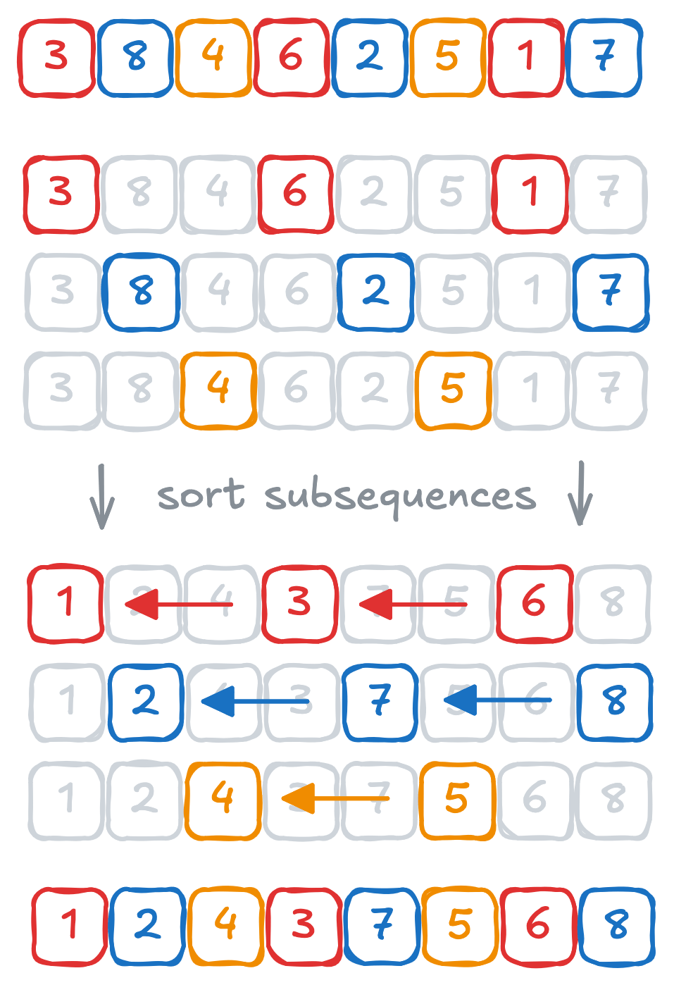
After this step we say the array is $k$-ordered. This means that for all $i$ we have ${A[i] \leq A[i + k]}$. Nothing is (directly) known about the relative order of elements which aren’t separated by a multiple of $k$. Since everything is a multiple of $1$, we see that $1$-ordered is just… sorted.

There is a fascinating property of $k$-sorting that is key to how Shellsort operates:

Theorem 1. If an array is $h$-ordered and then it is $k$-sorted, it remains $h$-ordered as well.

It is surprisingly tricky to prove this simple statement. A proof sketch paraphrased from a formal proof due to Knuth (TAOCP, Vol. 3, Chapter 5.2.1, Theorem K) goes as follows:

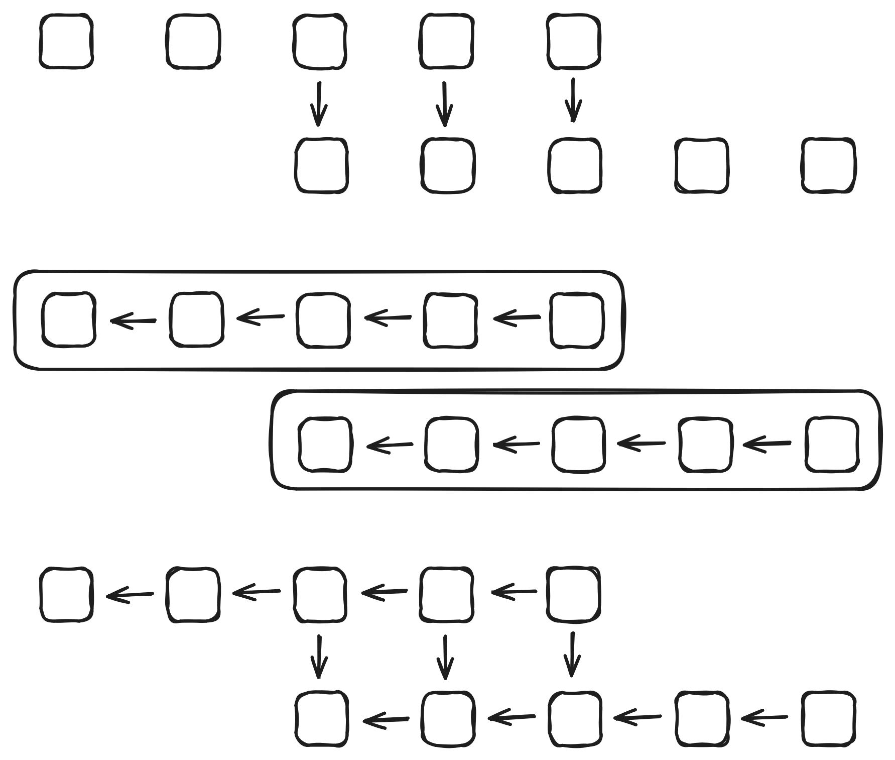
Lemma 1. If the last $r$ elements from array $Y$ are bigger or equal to respectively the first $r$ elements from array $X$, then this remains true after sorting both arrays.

Proof sketch. There are at least $r$ elements in $X$ which are smaller than or equal to elements in $Y$, thus the maximum element in $Y$ dominates at least $r$ elements, and thus the last element of $Y$ dominates the $r$th element of $X$ after sorting both. Apply a similar argument for $r - 1$ and the second largest element, etc.

A visual representation of this lemma really helps the understanding I believe:

Now we can use this lemma to prove our original theorem:

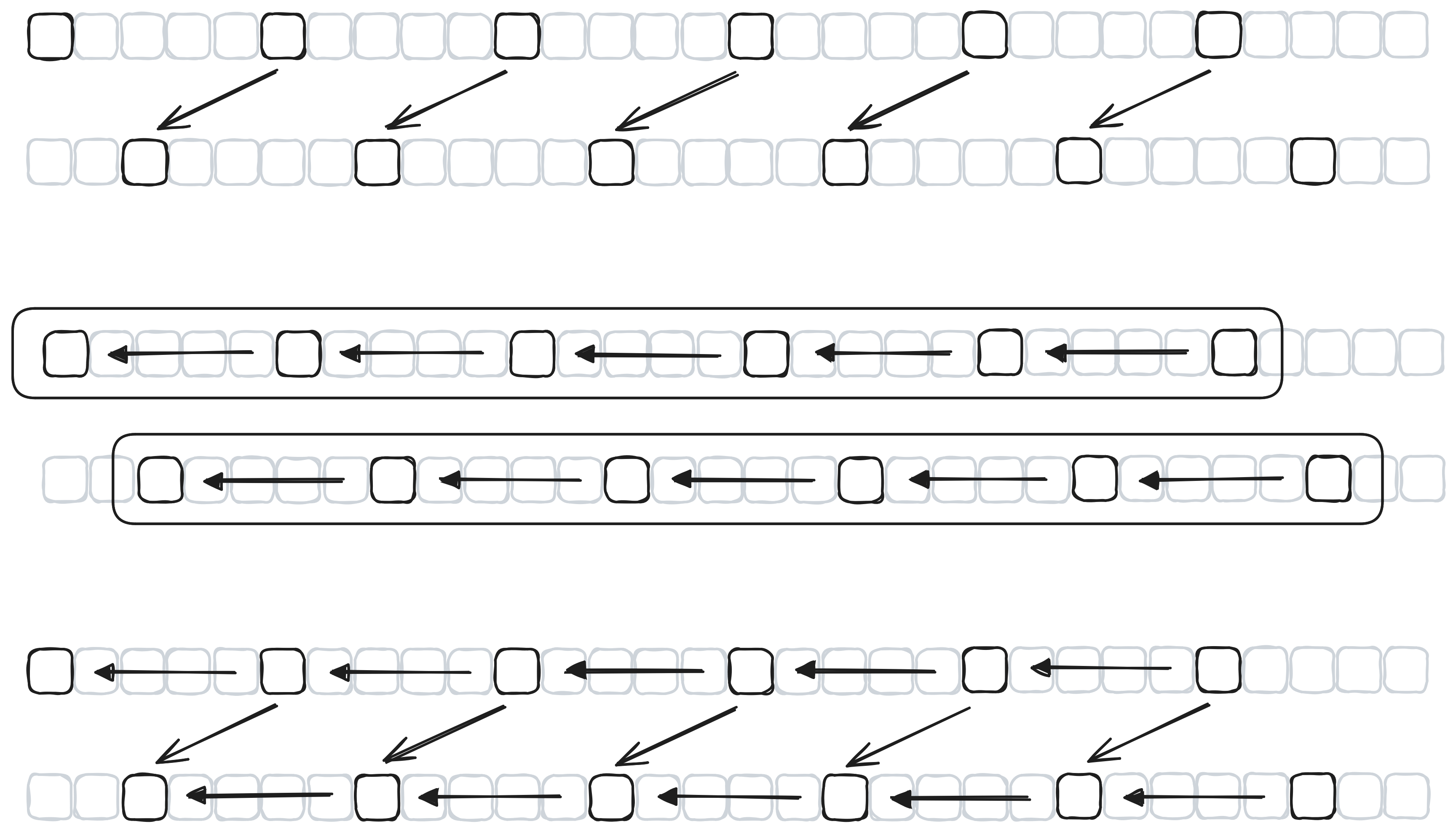
Proof sketch of Theorem 1. We have some array $A$ which is $h$-ordered, and thus we have $A[i] \leq A[i + h]$ for valid $i$. Then we $k$-sort it and now have $A[i] \leq A[i + k]$ instead. For any particular choice of $i$, define $X$ as $A[i + sk]$ for all valid integer $s$, and $Y$ as $A[i + tk + h]$ for all valid integer $t$. Then you can apply Lemma 1 to show that $A[i] \leq A[i + h]$ still remains true after $k$-sorting.

Once again I think a visual representation really helps here, especially to see the parallels with Lemma 1. Suppose we have a $3$-ordered array and then $5$-sort it. The proof sketch of Theorem 1 for $i = 2$ (and in fact for any $i \equiv 2 \pmod 5$) that we still have $A[i] \leq A[i + 3]$ can then be visualized as such:

I chose to only show a proof sketch rather than a full formal proof in this blog post, as I quote:

“This is much harder to write down than to understand.” — Donald Knuth

The result of this theorem is that as you apply more and more steps of $k$-sorting, all the work compounds into a larger overall ordering. Even with just two steps we can see very powerful results:

Lemma 2. If an array is both $h$-ordered and $k$-ordered where $k$ and $h$ are relatively prime (they don’t share any divisors other than 1), then two elements in the array which are at least $s \geq (h-1)(k-1)$ steps apart are in a correct relative order.

Proof. It is possible to write $s = \alpha h + \beta k$ with integer $\alpha, \beta \geq 0$ (for a proof of that see here). This means we can do $\alpha$ steps of $h$ (each time using $A[i] \leq A[i + h]$ since we’re $h$-ordered) and similarly $\beta$ steps of $k$ to see that $A[i] \leq A[i + \alpha h + \beta k] \leq A[i + s]$.

For example, here is a visualization of the relative order implied by the combination of $4$-ordering and $9$-ordering:

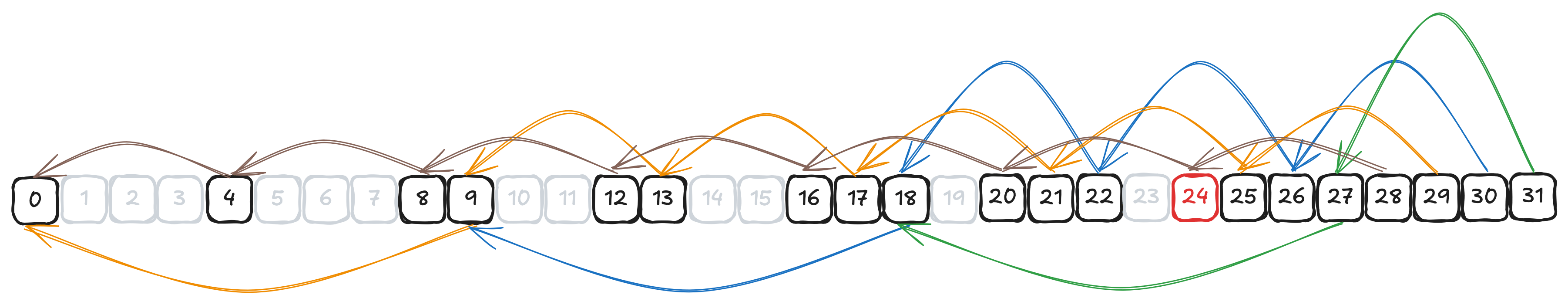
We see that indeed starting from offset $(4 - 1)(9 - 1) = 24$ each element is ordered relative to the element at 0.

More generally, we find that if we $k$-sort with some set $\{k_i, \dots, k_j\}$ and $\gcd(k_i, \dots, k_j) = 1$, then there exists some upper bound such that all numbers greater than it are representable as sums of non-negative multiples of $k_i, \dots, k_j$, meaning all elements beyond that point are ordered correctly relative to the starting point. Finding this upper bound is known as the Frobenius problem or coin problem, and it is a hard number theoretic problem. Some formulae like the above one for two coprime integers are known but the general problem for arbitrary sets of $k$ is NP-hard. It is this problem that forms the surprising link between Shellsort and number theory which will ultimately lead us towards the Fibonacci numbers.

Insertion sort

Shellsort uses insertion sort to $k$-sort the subsequences. This sort repeatedly swaps the last unsorted element with the element before it until it falls into place before continuing with the next unsorted element. This is generally speaking a rather inefficient algorithm for large arrays, as it has a worst-case of $O(n^2)$. However, this worst-case complexity can be refined. If each element is at most $m$ steps away from its final sorted position, insertion sort takes $O(nm)$ time.

And this is the key to Shellsort’s subquadratic worst-case complexity. You choose a clever gap sequence such that gaps start off very large leading to small subsequences and thus small $O(n^2)$ terms. Then, when Shellsort starts $k$-sorting with smaller gaps, you can use the fact that no element is very far from its final position to prove that it is still efficient. For example, based on our earlier observations, if the array is $4$-ordered and $9$-ordered and we do a $1$-sort (that is, a regular sort with no gaps) we know insertion sort can not run slower than $O(24n) = O(n)$ because each element is no further than $m = 24$ steps away from its final position.

Gap sequence

Choosing the gap sequence is thus key to Shellsort’s performance. The Wikipedia page lists many known gap sequences with different complexities. For example Hibbard’s 1963 sequence $k_i = 2^{i} - 1$ with $O(n^{3/2})$ complexity, or Pratt’s from 1971 which chooses all numbers of the form $2^p3^q$ for a complexity of $O(n\,(\log n)^2)$ (still the best known sequence to date, at least asymptotically).

However, all ‘new’ sequences listed after 1986 are empirically established, their complexities are unknown. They perform very well in practice, but they could possibly have much slower than expected performance for some inputs. A search on Google Scholar reveals no interesting new sequences either. With that in mind I’m happy to announce that Shellsort with the gap sequence

$$k_i = F_i \cdot F_{i+1} = (1, 2, 6, 15, 40, 104, 273, \dots)$$

where $F_n$ is the $n$th Fibonacci number has a worst-case runtime of $O(n^{4/3})$.

An interesting Fibonacci property

Before we can prove this worst-case runtime of gap sequence we’re going to need to take a look at the Fibonacci numbers in more detail:

$$F_0 = 0, \quad F_1 = 1, \quad F_n = F_{n-1} + F_{n-2}$$

This very well-known series of numbers $0, 1, 1, 2, 3, 5, 8, 13, \dots$ has all kind of interesting properties, but today we’ll need a very curious property where for $a, b > 0$, $$\gcd(F_a, F_b) = F_{\gcd(a, b)},$$ where $\gcd$ is the greatest common divisor function.

This property in plain words states that the greatest common divisor of the $a$th and $b$th Fibonacci number can be found by computing the greatest common divisor of $a$ and $b$, and looking up that index in the Fibonacci series.

Addition formula

To prove that we first need to prove the addition formula of the Fibonacci numbers, where $n, m > 0$, $$F_{n+m} = F_{n+1}F_m + F_nF_{m-1}.$$ A fairly simple way to do this is using the matrix exponential form of the Fibonacci sequence, $$\begin{pmatrix}F_{n+1}&F_n\\F_n&F_{n-1}\end{pmatrix} = {\begin{pmatrix}1&1\\1&0\end{pmatrix}}^n.$$

This form can be easily proven as correct using induction. With $n = 1$ you can directly see the equality holds, and to prove it holds for $n + 1$ assuming it holds for $n$ we have

\begin{align*} {\begin{pmatrix}1&1\\1&0\end{pmatrix}}^{n + 1} &= {\begin{pmatrix}1&1\\1&0\end{pmatrix}}{\begin{pmatrix}1&1\\1&0\end{pmatrix}}^n = {\begin{pmatrix}1&1\\1&0\end{pmatrix}}\begin{pmatrix}F_{n+1}&F_n\\F_n&F_{n-1}\end{pmatrix}\\ &= \begin{pmatrix}F_{n+1}+F_{n}&F_n+F_{n-1}\\F_{n+1}&F_{n}\end{pmatrix} = \begin{pmatrix}F_{n+2}&F_{n+1}\\F_{n+1}&F_{n}\end{pmatrix}. \end{align*}

Then, using the fact that in matrix exponentiation $A^{n+m} = A^n \times A^m$ we find:

\begin{align*} \begin{pmatrix}F_{n+m+1}&F_{n+m}\\F_{n+m}&F_{n+m-1}\end{pmatrix} &= \begin{pmatrix}F_{n+1}&F_n\\F_n&F_{n-1}\end{pmatrix} \times \begin{pmatrix}F_{m+1}&F_m\\F_m&F_{m-1}\end{pmatrix}\\ &= \begin{pmatrix}F_{n+1}F_{m+1}+F_nF_m&F_{n+1}F_m+F_nF_{m-1}\\F_nF_{m+1}+F_{n-1}F_m&F_nF_m + F_{n-1}F_{m-1}\end{pmatrix}. \end{align*}

Our desired addition formula can then be read from the top right element of both sides of the matrix equation.

If we generalize the Fibonacci formula a bit to allow negative indices we find that $F_{-1} = 1$ (which is the only choice preserving $F_{n} = F_{n-1} + F_{n-2}$), and that the above addition formula also holds for $n > 0, m = 0$ which we’ll need in a bit.

Divisibility and coprimality

We also need to prove that $F_{kn} \equiv 0 \bmod F_{n}$ for all $k, n > 0$. If we do induction on $k$ it obviously holds true for $k = 1$, and we see that if it holds for $k$ we have \begin{align*} F_{(k + 1)n} \equiv F_{kn + n} &\equiv F_{kn+1}F_{n} + F_{kn}F_{n - 1}\\ &\equiv F_{kn+1} \cdot 0 + 0 \cdot F_{n - 1} \equiv 0 &&\mod F_{n}. \end{align*} In other words, $F_n$ divides $F_{kn}$, also written $F_{n} \mathrel{|} F_{kn}$.

Finally we need to prove that $\gcd(F_n, F_{n+1}) = 1$, meaning consecutive Fibonacci numbers don’t share any prime factors (they are coprime). This is once again proven through induction, the property holds for $n = 1$ and since $\gcd(a, b) = \gcd(a, a + b)$, we have $$\gcd(F_n, F_{n+1}) = \gcd(F_n + F_{n+1} , F_{n+1}) = \gcd(F_{n+1}, F_{n+2}).$$

Euclidean algorithm

The Euclidean algorithm is an algorithm to compute the greatest common divisor based on the identity $$\gcd(a, b) = \gcd(a, b - a),$$ where $1 < a < b$. By repeatedly applying this identity (swapping $a, b$ when needed to keep $a < b$) until $a = 1$ you’ll find the greatest common divisor. You can speed up the algorithm by replacing the repeated subtraction with the modulo operator: $$\gcd(a, b) = \gcd(a, b \bmod a).$$

Now, suppose we are computing $\gcd(F_a, F_b)$ with $0 < a < b$. We can write $b = qa + r$ with $q \geq 1$ and $0 \leq r < a$, this is just splitting up $b$ into the quotient $q$ and remainder $r$ when dividing by $a$. Then, using the addition formula we find

$$\gcd(F_a, F_b) = \gcd(F_a, F_{qa + r}) = \gcd(F_a, F_{qa + 1}F_r + F_{qa}F_{r-1})$$

We proved earlier that $F_{qa} \equiv 0 \mod F_a$, so applying the above modular identity we can eliminate the $F_{qa}F_{r-1}$ term, $$\gcd(F_a, F_b) = \gcd(F_a, F_{qa + 1}F_r).$$ We also know that $F_{qa+1}$ and $F_{qa}$ are coprime. Since all factors of $F_a$ are factors of $F_{qa}$ we can conclude that $F_a$ and $F_{qa+1}$ share no (prime) factors either. This property lets us eliminate that factor from the greatest common divisor calculation entirely: $$\gcd(F_a, F_b) = \gcd(F_a, F_r).$$

Since $r = b \bmod a$ we note the following symmetry when $1 < a < b$:

$$\gcd(a, b) = \gcd(a, b \bmod a),$$ $$\gcd(F_a, F_b) = \gcd(F_a, F_{b \bmod a}).$$

In other words, by repeatedly applying the above identity we can perform the Euclidean algorithm on the indices of the Fibonacci numbers, giving $$\gcd(F_a, F_b) = F_{\gcd(a, b)}.$$

Fibonacci sort’s complexity

Now, for the actual proof I have to stand on top of the shoulders of giants. Recall that our gap sequence was as follows:

$$k_i = F_{i} \cdot F_{i + 1}.$$

In the 1986 paper A New Upper Bound for Shellsort by Robert Sedgewick, a formula due to Johnson is shown (Theorem 4) which lets us bound the Frobenius term $g(a, b, c)$ for three numbers $a, b, c$, assuming that they are independent. The Frobenius term $g(a, b, c)$ is what we discussed earlier in our analysis of Shellsort. It means that for all $n \geq g(a, b, c)$ there exist some combination of non-negative integers $\alpha, \beta, \gamma$ such that $$\alpha a + \beta b + \gamma c = n.$$

Conversely, independence means none of the numbers can be written as a linear combination of the others with non-negative integer coefficients. Assuming $i \geq 2$, for $\{k_i, k_{i+1}, k_{i+2}\}$ it is easy to prove the independence using our earlier GCD formula. From this we establish that $$\gcd(F_{i}, F_{i+1}) = F_{\gcd(i, i+1)} = F_{1} = 1,$$ $$\gcd(F_{i}, F_{i+2}) = F_{\gcd(i, i+2)} = F_{2} = 1,$$ and thus $$\gcd(k_{i}, k_{i+1}) = \gcd(F_{i}\cdot F_{i+1}, F_{i+1}\cdot F_{i+2}) = F_{i+1}\cdot \gcd(F_{i}, F_{i+2}) = F_{i+1}.$$ This directly proves that $k_{i+1}$ is not a multiple of $k_{i}$. This leaves one other possibility, that $k_{i+2}$ is dependent on $\{k_i, k_{i+1}\}$: $$\alpha k_{i} + \beta k_{i+1} = k_{i+2}$$ $$\alpha F_i F_{i+1} + \beta F_{i+1} F_{i+2} = F_{i+2}F_{i+3}$$ $$F_{i+1}(\alpha F_i + \beta F_{i+2}) = F_{i+2}F_{i+3}$$ This can only be true if $F_{i+2}F_{i+3}$ is a multiple of $F_{i+1}$, but $F_{i+1}$ is coprime with both $F_{i+2}$ and $F_{i+3}$ as we saw earlier, and thus this rules out any dependence.

Frobenius bound

Since we have proven independence we can use Johnson’s formula from the above paper. It states that $$g(a, b, c) = d \cdot g\left(\frac{a}{d}, \frac{b}{d}, c\right) + (d-1)c$$ where $d = \gcd(a, b)$. This lets us use the formula for coprime $a, b$ we saw in Lemma 2, because when $a, b < c$ and $a, b$ are coprime we have $$g(a, b, c) \leq g(a, b) = (a - 1)(b - 1) \leq ab.$$ In our case this means that $$g(k_{i+1}, k_{i+2}, k_{i+3}) \leq F_{i+2} \cdot g(F_{i+1}, F_{i+3}) + F_{i+2}F_{i+3}F_{i+4},$$ $$g(k_{i+1}, k_{i+2}, k_{i+3}) \leq F_{i+1}F_{i+2}F_{i+3} + F_{i+2}F_{i+3}F_{i+4}.$$ If we now use the asymptotic approximation $F_n = \Theta(\phi^n)$ where ${\phi = (\sqrt{5} + 1)/2}$ we have

$$k_i = \Theta(\phi^{2n}), \quad g(k_{i+1}, k_{i+2}, k_{i+3}) \leq \Theta(\phi^{3n}).$$

In other words, $g(k_{i+1}, k_{i+2}, k_{i+3}) = O(k_i^{3/2})$.

Back to Shellsort

We proved just above that after having processed gaps $k_{i+3}, k_{i+2}, k_{i+1}$ the maximum distance for an element from its true location is no more than $O(k_i^{3/2})$. Then if we perform a $k_i$-sort next, we have $k_i$ subsequences of length $n / k_i$ in which the maximum distance of an element from its sorted location within that subsequence is no more than $O(k_i^{3/2} / k_i) = O(k_i^{1/2})$.

Recall from earlier that insertion sort on a subsequence of length $n$ where each element is at most $m$ places from its sorted location has complexity $O(nm)$. This means the $k_i$-sort step for all subsequences combined takes at most $O(k_i \cdot (n / k_i) \cdot k_i^{1/2}) = O(n \cdot k_i^{1/2})$ time. This bound is good when $k_i$ is small, but we also have a different upper bound which is good when $k_i$ is big, using the fact that insertion sort takes at most $O(n^2)$ time. This gives us the bound $O(k_i \cdot (n / k_i)^2) = O(n^2 / k_i)$ as well.

We note that both bounds are equal when $k_i = \Theta(n^{2/3})$, giving us $O(n^{4/3})$ overall by consistently choosing the smaller of the two bounds. To make this a bit more formal, let $t$ be the maximum index such that $k_t \leq n$, and let $s$ represent the index on which we switch our bound. Then we have $$cT \leq \sum_{i=1}^{s - 1} \left(n \cdot k_i^{1/2}\right) + \sum_{i=s}^t \left(n^2 / k_i\right),$$ where $T$ is our total runtime and $c > 0$ is some ‘constant’ irrelevant for the asymptotic analysis (varying from equation to equation). Then, substituting the asymptotic approximation for $k_i \approx \phi^{2i}$ we get $$cT \leq n \sum_{i=1}^{s - 1} \phi^{i} + n^2\sum_{i=s}^t \phi^{-2i},$$ $$cT \leq n \cdot \frac{\phi^s - \phi}{\phi - 1} + n^2 \cdot \frac{\phi^{2 - 2s} - \phi^{-2t}}{\phi^2 - 1}.$$ Removing constant factors from terms and substituting $s = 2t/3$ gives us $$cT \leq n \cdot (\phi^{2t/3} - 1) + n^2 \cdot (\phi^{- 4t/3} - \phi^{-2t}).$$ Finally we note that within a constant factor $\phi^{2t} \approx k_t \approx n$ to simplify to $$cT \leq n \cdot (n^{1/3} - 1) + n^2 \cdot (n^{- 2/3} - 1/n),$$ $$cT \leq n^{4/3} + n^{4/3} - 2n,$$ giving our overall bound of $O(n^{4/3})$.

Generalizing

The above proof is analogous to the one found in A New Upper Bound for Shellsort by Sedgewick, I don’t claim credit for it. Ultimately there is nothing fundamental about the choice of the Fibonacci numbers here, any sequence which starts with $1$ and:

1. grows like $\Theta(b^{2n})$ for some base $b$,
2. has a greatest common divisor on the order of $\Theta(b^n)$ for consecutive terms, and
3. where any three consecutive terms are independent,

should have a $O(n^{4/3})$ runtime when used as a gap sequence in Shellsort. For example, Sedgewick himself used (among others) the sequence $$k_1 = 1, \quad k_i = (2^i - 3)(2^{i+1} - 3),$$ but it is pretty neat that the product of consecutive Fibonacci numbers can be used here as well.

In fact, we can generalize our Fibonacci sequence to a simple way of constructing sequences that match the above set of criteria. Simply start with a sequence $A_n$ where any three consecutive elements of $A$ are pairwise coprime and grow like $\Theta(b^n)$, then define the gap sequence as $$k_i = A_i \cdot A_{i+1}.$$

Real-world performance

So… is Fibonacci sort any good in practice? As far as shellsorts go, it is middle-of-the-pack. I also found a similarly structured sequence (with a similar $O(n^{4/3})$ proof) which performs quite a bit better:

$$A_1 = 1, \quad A_2 = 2,\quad A_n = 2A_{n-2} + 1$$ $$k_i = A_i \cdot A_{i+1}$$

The advantage of this gap sequence, like the Fibonacci one, is that it is a simple reversible recurrent formula meaning the implementation does not need a lookup table, and can compute the gaps on-the-fly. This is useful, because in my opinion Shellsort only truly has one niche where it shines: tiny code size. I think it’s a solid choice for places where every byte of code matters, while still giving a decent algorithm.

I ran a simple benchmark for the number of comparisons performed by the following gap sequences:

I also added heapsort as a $O(n \log n)$ comparison datapoint as it too is a small in-place unstable sort. The results are as follows, with a log scale for size $n$ on the X-axis and the number of comparisons divided by $n \log_2 n$ on the Y-axis:

As you can see fib25 doesn’t perform great nor terrible. My other sequence orlp25 performs almost as good as the best experimentally derived sequences, but still provides a worst-case guarantee.

Knuth Reward Check

The astute observer may have seen sedge86i marked as having an unknown complexity in bold. However, the Wikipedia page for Shellsort at the time of writing lists it as $O(n^{4/3})$. While writing this article I did quite some reading of Sedgewick’s 1986 paper A New Upper Bound for Shellsort, in fact I originally found the paper through a reference on the Wikipedia page for that sequence.

While reading the paper I noticed that there are two theorems he proves both of which lead to $O(n^{4/3})$ behavior, Theorem 5 and Theorem 6. Theorem 5 requires as a key property that $k_i, k_{i+1}$, and $k_{i+2}$ are pairwise coprime for all $i$. Theorem 6 requires as a key property that the greatest common divisor of consecutive terms $k_i, k_{i+1}$ always is on the order of $\sqrt{k_i}$ (that’s the theorem I used above).

But sedge86i which consists of the merger of two sequences satisfies neither property, nor do the individual sequences before merging!

\begin{align*} \{4^j - 3\cdot 2^j + 1\} &= 5, 41, 209, 929, 3905, 16001, 64769, 260609, \dots\\ \{9\cdot 4^j - 9\cdot 2^j + 1\} &= 1, 19, 109, 505, 2161, 8929, 36289, 146305, 587521, \dots \end{align*}

As counterexamples in the pre-merged sequences we find $\gcd(209, 3905) = \gcd(36289, 587521) = 11$, and $\gcd(16764929, 37730305) = 29$ in the merged sequence. In fact, if you read the paper, Sedgewick only describes the merged sequence in his conclusion section, as such:

The particular sequence used here is a merge of the sequences […]. These occasionally have triples that are not relatively prime, but the combination does better on random inputs than the sequence of Theorem 5 because it has more smaller increments.

Sedgewick never claims this particular merged sequence leads to a worst-case of $O(n^{4/3})$. So why is it listed as such on the Wikipedia page? After more digging I realized that the sequence is also found in Knuth’s TAOCP, in Volume 3, Sorting and Searching, Chapter 5.2.1. At the time Knuth wrote:

The final examples in Table 6 come from another sequence devised by Sedgewick, based on slightly different heuristics. When these increments $(h_0, h_1, h_2, \dots) = 1, 5, 19, 41, 109, 209, \dots$ are used, Sedgewick proved that the worst-case running time is $O(N^{4/3})$.

Except Sedgewick did no such thing (nor did he claim to). I guess whoever edited the Wikipedia article read Knuth’s book and assumed that statement was correct.

Contacting Knuth

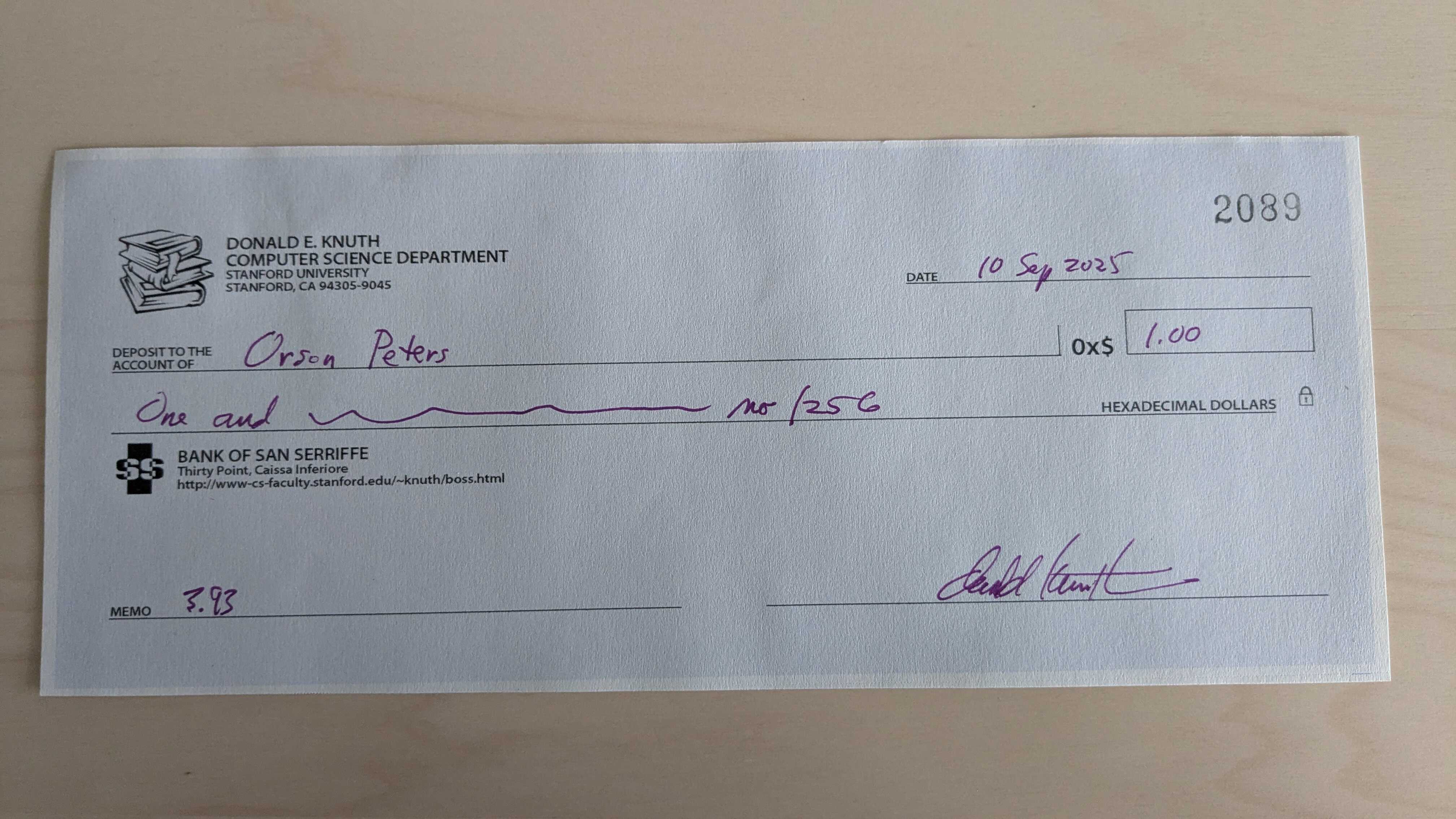
I emailed Knuth with my findings, and a good few months later I received a physical letter containing:

1. my email printed out with a few pencil scribbles,
2. a reward check for finding an error.

The errata for Volume 3 now read (emphasis mine):

These increments […] combine two sequences that resemble increments for which Sedgewick proved the worst-case time bound $O(N^{4/3})$.