Black-Box HashDoS: Attacking Hash Tables Without Knowing the Hash Function

In this article I will describe a novel technique that allows an attacker to pass attacker-chosen string keys to a hash table implementation such that each lookup query takes $O(n)$ instead of the expected $O(1)$ work. The attack takes $O(n \log n)$ interactive steps with the hash table to prepare, and does not require knowledge of the hash function used by the hash table. Instead, the technique directly targets the underlying structure of the hash table.

Luckily these attacks as described are quite niche (requiring lookup, insert and clear access on a table without interference from others), and mitigations are possible. However, the attack isn’t purely theoretical, I construct a working attack against Rust’s standard library hash table implementation below.

Since not everyone might be on the same page on hash table terms & notation, or are aware of previous attacks, I will describe those first, and then my attack.

Hash table basics

Hash tables are nifty data structures that use hash functions to efficiently map keys to values. There are hundreds of subtly different designs for hash tables, but they generally follow the same structure:

• They have a contiguous array, typically of length $B = 2^\ell$, of buckets. Each bucket contains a key, and a value.

• They have a hash function $h$ that maps a key $k$ to an integer in $[0, B)$, often through $h(k) \bmod B$. This integer gives the index of a bucket in our array. We’re going to abstract over this and just say this bucket is called $\operatorname{bucket}(k)$.

• During insertion, we look at $\operatorname{bucket}(k)$. If this bucket is empty, we place our key/value pair there. If it is not empty, we compare $k$ to the key that’s already there. If they’re equal, we replace the value with our new value. If they’re not equal we need to look at the next bucket and repeat until we find our key or hit an empty bucket.

• During querying we once again look at $\operatorname{bucket}(k)$. If the bucket is empty we return that our key is not in the hash map. If it isn’t empty we compare $k$ to the key in the bucket. If they’re equal, we return the value in the bucket, otherwise we once again need to repeat our procedure at the next bucket.

How do we know which bucket to look at next? There are two main strategies for this:

1. Chaining. In this variant a bucket contains a pointer to the next bucket to inspect, with this bucket being allocated outside our main array, forming a linked list. Sometimes the main array doesn’t contain keys/values at all and only contains pointers, pointing to the first bucket to inspect.

2. Open addressing. In this variant there is some function $\operatorname{probe}(b, i)$ that takes initial bucket $b = \operatorname{bucket}(k)$ and zero-indexed step $i$, returning which bucket in our array to look at in step $i$. Two subvariants are by far the most common:

   1. Linear probing, using $\operatorname{probe}(b, i) = (b + i) \bmod B$.
   2. Quadratic probing, using $\operatorname{probe}(b, i) = \left(b + i^2\right) \bmod B$.

In this article we’ll be attacking open addressing, although chaining can similarly be attacked in $O(n^2)$ setup time.

The load factor is $n / B$, where $n$ is the number of elements we store in our hash map. For chaining a higher load factor simply increases the expected linked list length, which is fairly predictable. However, for open addressing there is a steep asymptote in performance cost for insertion and queries as the load factor approaches $1$. This is because the insertion/query algorithms require an empty bucket for termination, and as the load factor approaches $1$ it becomes harder and harder to find an empty bucket. For this reason open addressing schemes tend to increase $B$ and re-hash the hash table once the load factor approaches some constant close to $1$, like $0.8$.

Traditional HashDoS

Traditional HashDoS (from Denial of Service) is an algorithmic complexity attack that intends to make a hash table much slower than usual. First described in 2003 by Crosby and Wallach in “Denial of Service via Algorithmic Complexity Attacks”, the attack is conceptually incredibly simple: insert $n$ elements that all have the same hash value.

After doing this, if you search for another new value $x$ not found in the hash table with that same hash value, the implementation has to scan through all $n$ values before realizing this value doesn’t exist. This is $O(n)$ behavior for an operation we expect to execute in $O(1)$ if the hash function were truly random.

Surely you would expect every hash table implementation in common use to not be vulnerable to this attack from 2003, but alas. For example, the std::unordered_set implementation found in C++ is still vulnerable by default in libc++ and libstdc++ as they dispatch to MurmurHash and CityHash with a fixed seed. I’ve written about this extensively in Breaking CityHash64, MurmurHash2/3, wyhash, and more….

In languages like Rust and Python the hash table implementation protects against traditional HashDoS by default: they choose a hash function with a secret randomly initialized seed, making it hard to find values with the same hash.

A new gadget

The new approach we take here will be well familiar to someone in cryptography: a side-channel attack. For hash tables with string keys there is a crucial step that occurs during lookups, namely that the key has to be compared for equality, if a bucket is occupied.

And this gives us a gadget. By ensuring that all keys we insert start with a long common prefix (e.g. 'aaaaaa...aa0001', 'aaaaaa...aa0002') we can determine how many keys were compared for equality during a lookup if it also starts with the same prefix. This is because such an equality check has to check the entire common prefix which is going to take a while. If we start a stopwatch before a lookup and stop it afterwards we can infer how many times a key was compared by comparing the measured time to lookups that didn’t have such comparisons.

In turn, we can use this to derive information about which buckets are occupied when inserting what keys. We can then work backwards and construct sets of keys that occupy just the right buckets in the right order to create linear-time lookups.

In the rest of this article I will mention new_key() a bunch of times. I assume that this function always returns a completely unique key with a fixed length and a long common prefix.

Linear probing

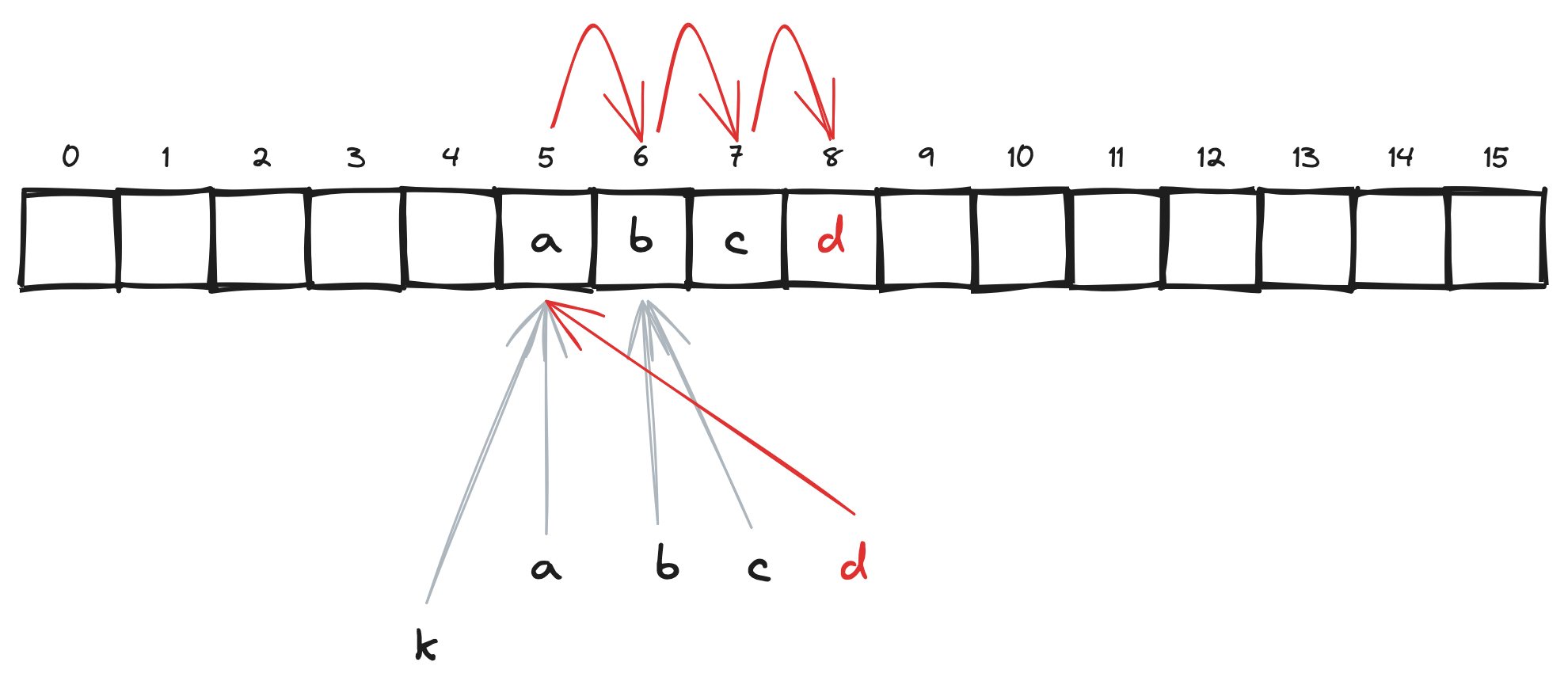
Linear probing is the easiest setup to attack. Recall that when using linear probing in case we don’t find our key in bucket $i$ we’ll look at bucket ${(i + 1) \bmod B}$, only stopping on an empty bucket. So if we can create a long chain of occupied buckets plus an extra key k not in the hash table that maps to the first bucket in that chain, any lookup for k will take time scaling with the length of the chain.

Without further ado, the attack:

1. Ensure that the hash table has $B$ buckets by inserting sufficiently many unique keys before clearing the table.

2. Insert one new_key() into the hash table.

3. Repeatedly do k = new_key() and lookup(k), until such a lookup causes a comparison. Save this k as detonator.

4. Keep creating new keys and looking them up in the hash table. Every time such a lookup causes comparisons, insert the key into the table. Do this until a total of $n$ elements are in the table, making sure $n/B$ stays below the load factor that would trigger a re-hash.

Now every time you do a lookup(detonator) the hash table has to look through a long chain of $n$ buckets to find that detonator is missing.

It’s possible (likely even) that an insert from step 4 initially tries inserting somewhere inside the chain, but due to the linear probing schedule always following the same path regardless of its starting location ($i$, $i+1$, etc.) its final insert location will always be at the end of the chain, extending it.

The total time complexity to set up this attack is $O(n \log n)$ (if $B \approx n$). It starts slow but speeds up towards the end. After step 3 there is one occupied bucket, so the first lookup that causes comparisons in step 4 takes $B$ iterations to find on average. However, the second lookup has two occupied buckets it can hit, so it will take $B / 2$ steps, the third $B / 3$, etc. In total you end up with $B \cdot (1/1 + 1/2 + \cdots + 1/n) = B H_n \approx n \log n$ steps, where $H_n$ is the $n$-th harmonic number.

Quadratic probing

Quadratic probing actually requires us to be far more clever to attack successfully, but perhaps somewhat surprisingly it’s also completely broken. In fact, the technique I’m about to show works for any probing scheme where the bucket we visit at step $i$ can be written as ${(\operatorname{bucket}(k) + f(i)) \bmod B}$ for any $f$, so long as we know $f.$

The attack will operate in four phases:

1. We will gather two sets of keys $S_1$ and $S_2$ such that each set covers each bucket exactly once.

2. We will establish a mapping between $S_1$ and $S_2$ so we know exactly which pairs map to the same bucket.

3. We will use $S_1$ and $S_2$ to find for each element $k \in S_1$ what its successor is, that is the element $k’ \in S_1$ such that $$\operatorname{bucket}(k) + f(1) \equiv \operatorname{bucket}(k’) \mod B.$$

4. From the successors and knowledge of $f$ we can derive the full order of the buckets (mod $B$), and create a hash table in which every bucket which would be visited by a lookup for some starting key $k$ is occupied.

Gathering sets of keys

First we will again ensure our hash table has $B$ buckets by inserting enough elements then clearing it. Here we’ll assume $B$ is a power of two, although these algorithms could be generalized. Then, we will create two pools of elements $X, Y$ by repeating the following step:

Generate a k = new_key(). Do a lookup(k), if it causes a comparison (meaning the bucket is occupied in the hash table) add it to set $X$, if $|X| < B/2$ insert it into the table and add it to $X$ as well, otherwise add it to $Y$.

The only reason we split this into two pools $X, Y$ is to prevent the hash table from re-hashing, which would happen if we filled it all the way up to $B$ elements.

We will do this until we have generated ‘sufficient’ elements such that random chance essentially guarantees we have two elements mapping to each bucket. This is a coupon collector’s problem. In this case (where we need two copies of each element) it’s also known as the double Dixie cup problem.

If we want to have at most an $\epsilon$ chance of failing to acquire $g$ copies of each element after sampling $s$ random keys, we can study the Chernoff bound on sums of Bernoulli variables. Let $U_i$ be the number of copies we have of an element mapping to bucket $i$ and let $\mu = s/B$. Then for $0 < \delta < 1$: $$\mathrm{Pr}[U_i \leq (1 - \delta)\mu] \leq \exp({-\delta^2\mu/2}).$$ If we let $(1 - \delta)\mu = g$ we get $$\mathrm{Pr}[U_i < g] \leq \exp\left(-\frac{\left(\mu - g\right)^2}{2\mu}\right),$$ after which a union bound over $B$ tells us that $$\mathrm{Pr}[\exists_i : U_i < g] \leq B \exp\left(-\frac{\left(\mu - g\right)^2}{2\mu}\right).$$ Sparing you the algebra exercise, if we substitute the left-hand side with $\epsilon$ we find that $$s \geq 2B \left (g + \ln \frac{B}{\epsilon}\right)$$ suffices.

So if we substitute $g = 2$ and, say, $\epsilon = 0.01$, we find how many keys we need to generate to ensure a 99% chance of success. After doing that and filling $X, Y$ we only need to uniquify and extract $X_1, X_2, Y_1, Y_2$.

To extract $X_1$ we clear the table and pop keys from $X$ one by one, doing a lookup for each. If a lookup causes a comparison we put it back into $X$ (this bucket is already covered but perhaps it’s still useful for $X_2$ later), otherwise we add it to $X_1$ and insert it into the table. We stop when $|X_1| = B/2$. We then repeat this process for the others. Finally, $S_1 = X_1 \cup Y_1$ and $S_2 = X_2 \cup Y_2$, each covering each bucket exactly once.

Establishing the mapping

We arbitrarily label the elements from $S_1, S_2$ with indices $0, 1, \dots, B - 1$ (making them arrays). We will also create an array mapping[idx2] = idx1 which for each element in $S_2$ contains the corresponding index of an element in $S_1$ which maps to the same bucket.

We initialize mapping to all zeros, then we do $\log_2 B$ iterations. In iteration $i$ we will clear the hash table then fill it with all keys from $S_1$ whose $i$-th bit in its index is set. This is at most half the elements, so the table won’t re-hash. Then (still in iteration $i$), we will do a lookup for each element in $S_2$ in order. If this causes a comparison to occur we know this element of $S_2$ shares a bucket with an element in $S_1$ that has the $i$-th bit set in its index. Therefore we set the $i$-th bit of its corresponding entry in mapping if this occurs, and otherwise we don’t.

Once this process is complete mapping[idx2] = idx1 will have been constructed precisely bit-by-bit for each element, in $O(B \log B)$ time. Using this mapping we shuffle $S_2$ so that from this point on we can assume the $i$-th elements of $S_1$ and $S_2$ map to the same bucket.

Finding successors

This process is very reminiscent of the previous one. We initialize an array successor[idx] to zeros and once again do $\log_2 B$ iterations.

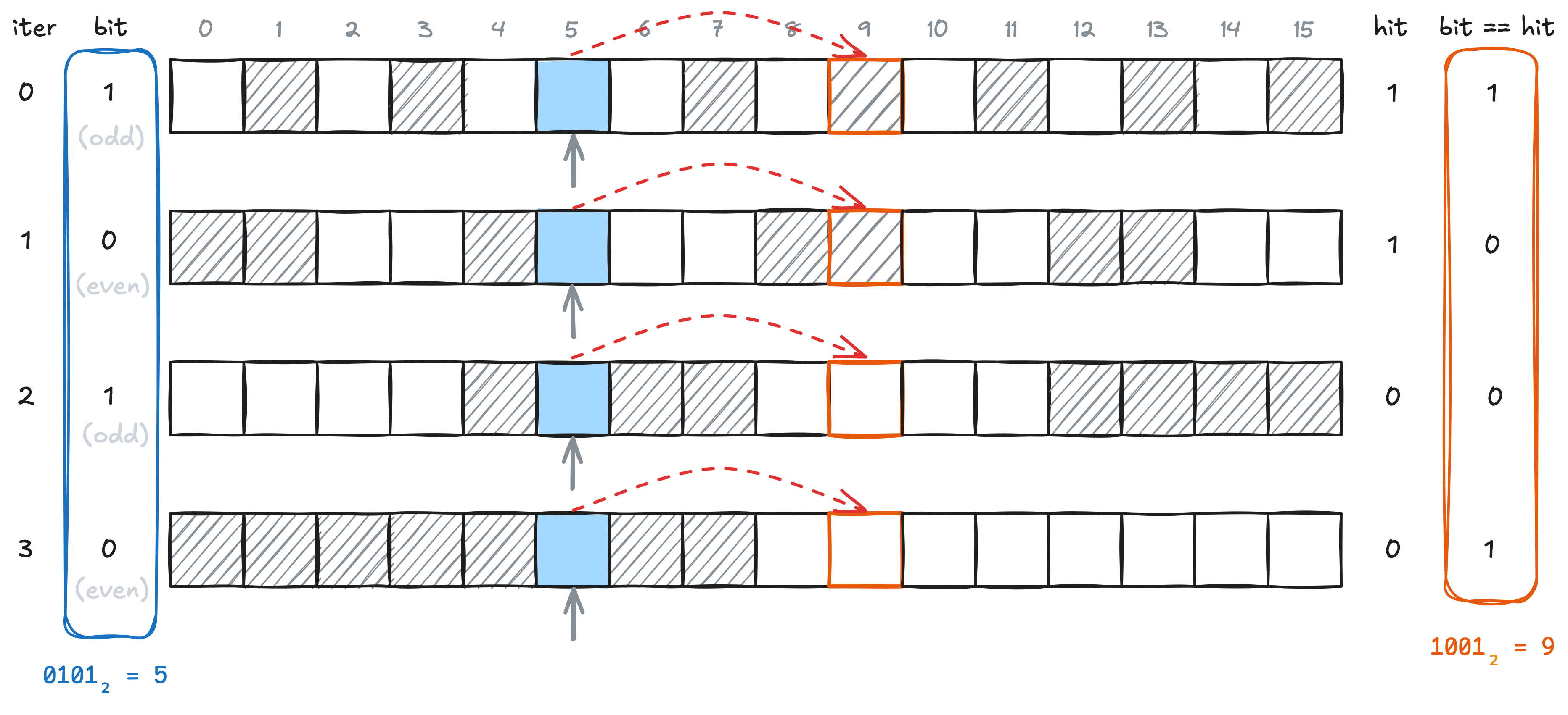
In iteration $i$ we first fill the table with just the elements in $S_2$ where the $i$-th bit of its index is $0$. Then we go through just the elements in $S_1$ whose $i$-th bit of their index is also $0$ and do a lookup for each. If this results in one comparison we know that the successor of this element is not in the table currently, and if it results in two or more comparisons we know it is. We set the $i$-th bit of their entry in successor accordingly. Then we repeat this process (still in iteration $i$) entirely analogously for those elements whose $i$-th bit of their index is $1$ to find the $i$-th bit of their successor as well.

Below is a visualization of how we can infer that the successor bucket of the element at index $5$ is the one at index $9$. Note that the buckets are shown in our current $S_1$/$S_2$ order, not the one in the hash table (which is the order we’re trying to find). The dashed red arrow is therefore the hidden information. Also note how either the odd or even blocks of buckets are filled based on whether the corresponding bit in $0101_2 = 5$ is set. We are thus only showing the half of each iteration that is relevant for $5$.

Finalizing the attack

Using our knowledge of $f(1)$ (which is simply $1$ in quadratic probing) and the successor table we can now re-order $S_1$, $S_2$ such that their order matches the buckets of the hash table precisely (at least cyclically mod $B$, we still don’t know which bucket truly is bucket $0$ in memory, but that doesn’t matter).

The attack is now trivial: clear the hash table and insert from $S_2$ the $n$ elements with index $0$, $f(1) \bmod B$, $f(2) \bmod B$, $\dots$, $f(n-1) \bmod B$. This is precisely the probing sequence the hash table will attempt when looking up the first element of $S_1$, causing it to take linear time to establish that it is not in the table.

Attacking hashbrown

Real-world hash tables can get more complicated still. For example the Rust library hashbrown, which also powers the standard library HashMap, has a different structure inspired by Abseil’s Swiss Tables.

In hashbrown, when doing a lookup for k, not only will bucket(k) be compared but in fact all occupied buckets in the window bucket(k)..bucket(k) + W will be compared, where $W$ is $8$ or $16$ depending on the platform. Each element also has a 7-bit tag derived from the hash which is compared before a string comparison occurs.

The latter problem is easy to overcome at a 128x slowdown of our attack. Instead of calling new_key() directly throughout the process we generate all the keys we’ll need upfront while the table still only has a single element in it, with a capacity of $< W$. This way we can detect if a comparison occurs which will directly imply the 7-bit tag matches.

The window lookup is both a blessing and a curse. We need a completely different algorithm, but can use the window lookup to extract information. The new algorithm has three phases: generating a covering (plus one extra ‘detonator’ element), inspecting the internal structure using the windows, and finding the bucket order of the covering.

Generating a covering

We want to generate a set $S$ of keys which maps to each bucket exactly once. We can still do this despite the $W$ window size. We initialize $S$ as the empty set and repeat the following process until $|S| = B$:

1. Clear the table and generate (or rather, pull from our pre-generated pool) $B / (2W)$ keys and insert them into the table iff lookup(k) causes no comparisons. The average distance between the buckets these keys map to will be $2W$, meaning most do not ‘see’ each other in their windows. Only a few will be discarded by the lookup check. Call the temporary set of kept keys $T$.

2. For each key in $S$ check if lookup(k) causes comparisons. Then clear the table and insert any $k \in S$ which caused comparisons earlier into the table. These are the keys that can ‘see’ at least one of the keys in $T$.

3. Do a lookup(k) for each $k \in T$. Add all keys $k$ for which the lookup did no comparisons to $S$.

Note that if two keys map to the same bucket they can always see each other. It should thus be easy to see the above process only adds keys with disjoint bucket(k) indices to $S$. The argument is a bit sophisticated, but this process will complete after an expected $O(W \log B)$ iterations, each iteration with $O(B)$ complexity.

Uncovering the structure

We will do a trick similar to the one from before in quadratic probing. We will assign an index $0 \leq i < B$ to each element in $S$ and then calculate, in a bit-by-bit fashion, for each element in $S$ the sum of all the indices of the elements in $S$ whose buckets lie in its window (excluding the index of each element itself). I think it’s easiest to just show the code for this one:

// Calculate sum of indices in window ahead of keys[idx].
let mut sum = vec![0; B];
for bit_idx in 0..B.trailing_zeros() {
    for bit in 0..=1 {
        // Put half the elements in the table.
        table.clear();
        for idx in 0..B {
            if (idx >> bit_idx) & 1 == bit {
                table.insert(keys[idx]);
            }
        }

        // For the other half, count number in the table that
        // lie within its window.
        for idx in 0..B {
            if (idx >> bit_idx) & 1 != bit {
                let in_table = lookup(table, keys[idx]);
                let in_window = if bit == 1 {
                    in_table
                } else { 
                    W - 1 - in_table
                };
                sum[idx] += in_window << bit_idx;
            }
        }
    }
}

This once again runs in $O(B \log B)$ time.

Finding the bucket order

We generate one more element not found in $S$, which we will call the detonator. This is the element we’ll end up performing lookups for, causing a traversal through the entire hash table for each lookup. Note that since $S$ is a cover over all buckets, exactly 1 element in $S$ maps to the same bucket as the detonator.

We clear the hash table and insert our detonator. Looping over $S$ we find all elements that have the detonator in their window, which should be precisely $W$ of them. Then by repeatedly clearing the table and inserting all but one of these elements followed by a lookup for the odd one out we can establish the order these elements should go in. E.g. the last one (which is positioned precisely at the detonator bucket) sees $0$ of the others, the one that sees $1$ of the others comes before that one, etc.

This establishes a starting point of $W$ fully ordered elements, anchored at the detonator location. We can now extend this iteratively over the full array using a clever trick:

let mut idx_of_bucket = /* the indices of the W starting elements */;
for i in 0..B-W {
    let next_idx = (sum[idx_of_bucket[i + 1]] + idx_of_bucket[i + 1]
                  - sum[idx_of_bucket[i]]);
    idx_of_bucket.push(next_idx);
}

Since we have at least two consecutive elements, those index sums we calculated earlier allow us to precisely deduce what the index of the next element is, by canceling out the consecutive sums.

Finalizing the attack

With the full bucket order decoded, the attack merely consists of inserting the keys for exactly the buckets that would be visited during a probe for the detonator, and (repeatedly) looking up the detonator element.

I have a working attack against hashbrown in ~200 LOC that can be found on the Rust playground. Note that here I replaced the timing attack in lookup with a direct comparison counter for illustration purposes and to make the demo deterministic, but for sufficiently long common prefix string keys a timing attack is able to do the exact same.

Mitigating the attack

We already saw that comparing a 7-bit tag before doing a string comparison slows the initial element generation down by a factor of $2^7$. So comparing a full 64-bit hash before comparing string keys completely stops all variations of this attack that I can think of.

It’s unclear if different probing schedules are safe, e.g. probing schemes where the order of probing depends on the hash in a non-linear way. I’ve only developed this attack as a proof-of-concept, other structures may be vulnerable as well.

It’s also unclear if this attack can be done without access to all of lookup, insert and clear, or in the presence of any other users of the hash table. I would be wary of relying too much on the impracticality of the attack due to these requirements however, as it may be possible more sophisticated side-channel attacks are able to resolve information despite other users and/or tombstones, e.g. using just insert and remove.